[Poster: html, pdf]

A good part of today’s internet content is created and shaped for delivering advertisements. Internet pages are interconnected by links, and a visitor is likely to open multiple pages from the same publisher. After a while, visitors leave the web site, either due to clicking on an advertisement or just because they get bored and switch to other content or activity.

The probability distribution of the session depth — the number of pages opened during a single visit — is an important metric for the publisher. It is used both to estimate revenues from the advertising campaign and to optimize the web site: links between pages, page content, and advertisements appearing on each page. Session depth constitutes a counting time series. There are established techniques for forecasting in counting time series, however those techniques are mostly based on assumption that the time series realizes a unimodal distribution at every point in time, such as the Poisson or the Geometric distribution. This assumption is inadequate for session depth time series: there are usually multiple pages where the visitor is most likely to leave; this commands a multi-modal predictive distribution.

A sequence of Beta-Bernoulli distributions, one for each page, gives a reasonable generative model for session depth. There are of course dependencies between pages — a user which is likely to leave on a certain page is also likely to leave on ‘similar’ pages, — but we can ignore these dependencies in an initial approximation. One phenomenon should be accounted for though — the website evolves as new pages are published, existing pages edited, and links between pages are added or removed. The posterior distribution should incorporate uncertainty due to such changes.

The Generative Model of a Visit

We view a visit as a sequence of opened pages of length at most $N$. A Beta-Bernoulli distribution $Beta\mbox{-}Bernoulli(\alpha_i, \beta_i)$ for the $i$th page for each $i \in {1, \ldots, N}$ models the event of leaving after visiting the page. We draw the session depth by passing through the sequence until the ‘left’ event (Algorithm 1).

Algorithm 1: Drawing the session depth

To update the beliefs based on the observed session depth $K$, we just increment $\beta_i$ if the visitor continued to the next page, that is $i < K$, or $\alpha_i$ if the visitor left at the $i$th page ($i = K$). We must also account for the uncertainty due to content changes (we are not informed about the changes). After trying a few alternatives, we represent uncertainty as a cap $C$ on the amount of evidence which we collect for each page. If $\alpha_i + \beta_i$ exceeds $C$ after updating, we scale down both $\alpha_i$ and $\beta_i$ by the same factor, such as the probability of leaving remains the same, but $\alpha_i + \beta_i$ is equal to $C$ (Algorithm 2).

Algorithm 2: Updating the beliefs based on the observed session depth.

The animation below shows running the model on 1000 visits, where the average session depth gradually decreases from 5 to 1. Note how the mean gradually and smoothly follows the trend, despite very noisy data. $C$ was set to 1000.

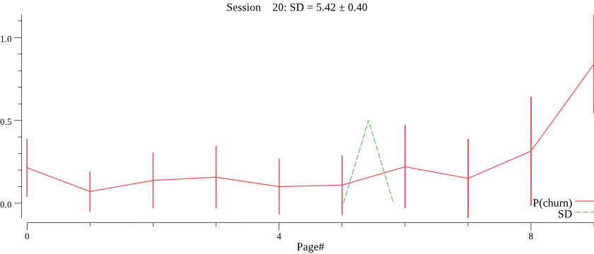
Obviously, we do not know the value of $C$ and want to infer $C$ for each campaign based on observed session depth counts. The right value of $C$ is crucial for the best forecasting performance, notice how a smaller value of $C$ ($C=30$) affects prediction of the session depth on the same data:

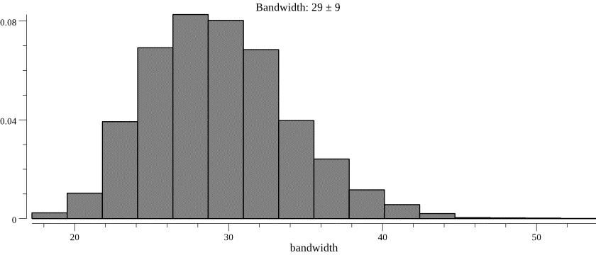
We turn to probabilistic programming for this task, putting a prior on $C$ and running the inference on the history of session depth observations. We then infer the posterior distribution of $C$, and use the mean of the posterior for forecasting. An example of predicted $C$ values is in the histogram below.

Probabilistic programs

The program code is at bitbucket.org/probprog/ppv-pp-paper, in the worksheets folder.

Prototype in Anglican

For prototyping, we used Anglican. The model is straightforward to implement in Anglican, a Lisp dialect. Since we only have a single random variable to infer, Metropolis-Hastings Monte Carlo performs well, and Anglican runtime is fast enough to produce 10,000 samples in 8 seconds, given 100 observations. However, there were reasons that prevented us from using Anglican in production, and we turned to other probabilistic programming environments.

Namely, we looked for Python API, scalability, and support for efficient variational inference; Edward and Pyro were two obvious candidates.

Implementation in Edward

Edward is based on TensorFlow and uses TensorFlow API for expressing flow control and variable updating. This results in more verbose code which is hard to read and debug. However, even when the challenge of expressing belief updates through tensor manipulations is overcome, an additional difficulty arises due to the complete separation between the generative model and the data in Edward. Our probabilistic program both conditions the distribution of $C$ and updates beliefs of leaving the article at each page based on the data. Specifying the model in a data-agnostic way is possible but inference would becomes unreasonably inefficient. In our simple case, belief updating and drawing the session depth can luckily be disentangled — the probability of leaving the campaign at each page does not depend on the updated beliefs for earlier pages. However, we still need to pass the data twice — both to the model and to inference.

Edward supports both Metropolis-Hastings and variational inference. Metropolis-Hastings gave results consistent with the Anglican implementation. One would expect static graph, C++-based implementation of Metropolis-Hastings to run much faster than in Anglican, however due to complex code having to go through tensor manipulations, the performance was quite poor — Edward draws 10,000 samples in about 6 minutes, more than 50 times slower than Anglican. At the time of writing, the implementation of variational inference in Edward has a limitation preventing its application to our model.

Implementation in Pyro

Pyro lets writing probabilistic programs in regular Python, almost without limitation. Python is definitely sufficient for implementing our probabilistic program. For inference, Pyro supports importance sampling and variational inference, along with other approaches.

We first ran the inference with importance sampling, which gave acceptable results, partially because our prior on $C$ was close to the posterior. However, the running times were even longer than with Edward: it takes more than 10 minutes for Pyro to draw 10,000 samples. We then turned to variational inference, only to discover that the model would have to be rewritten: since gradients are computed by the underlying PyTorch code, all involved computations must be expressed as non-destructive tensor manipulations, in a way similar to Edward implementation. Variational inference gave results consistent with importance sampling, however the learning rate had to be set low enough to ensure convergence. Consequently, the running time of variational inference was longer than of importance sampling for similar accuracy.

Final Solution: A Go Program

The full Go implementation is at http://bitbucket.org/dtolpin/pps.

Go is a (relatively) new programming language from Google. Recently, Go is increasingly used for machine learning and data science. We implemented the model in Go and manually coded a simple version of Metropolis-Hastings inference algorithm. The implementation came out amazingly lean and simple:

Updating beliefs

 1
 2
 3
 4
 5
 6
 7
 8
 9
10
11
12
13
14
15
16
17
18
19
20
21

func (m *Model) Update(bandwidth float64, count int) {
    for i := 0; i != len(m.Beliefs); i++ {
        var j int // selects either alpha or beta
        if i < count-1 {
            j = 1
        } else {
            j = 0
        }
        m.Beliefs[i][j]++
        // if the evidence exceeds the bandwidth, scale down
        evidence := m.Beliefs[i][0] + m.Beliefs[i][1]
        if evidence > bandwidth {
            scale := bandwidth / evidence
            m.Beliefs[i][0] *= scale
            m.Beliefs[i][1] *= scale
        }
        if j == 0 { // reached the last page of the session
            break
        }
    }
}

Metropolis-Hastings sampling

 1
 2
 3
 4
 5
 6
 7
 8
 9
10
11
12

func MH(query Query, proposal Proposal, x float64, samples chan<- float64) {
    logp := query.Observe(x)
    for {
        samples <- x
        x0, logp0 := x, logp
        x = proposal.Propose(x)
        logp = query.Observe(x)
        if logp-logp0 < math.Log(1.-rand.Float64()) {
            x, logp = x0, logp0
        }
    }
}

The implementation produces 10,000 samples for 1000 observations (ten times more data than for the probabilistic programs above) in less than a second, and the simulator runs blazingly fast. Animation gifs in this post were produced using the Go program, it would take too long to generate them with other tools.

Round-up

For deployment in production, we implemented a custom solution in Go, which is fast and works well for our current setup. The performance is much better than of any probabilistic system’s implementation. However, this impedes our ability to extend the probabilistic model to encounter for other factors and dependencies.

This case study points at properties of probabilistic programming systems which are crucial for adoption but missing in many of the implementations.

• Data structures must transparently support persistent updating and manipulation along with high performance.
• Automatic differentiation algorithms which work well for deep learning are not necessarily good enough for probabilistic programming.
• Small programs must run with acceptable performance.