Gaussian processes are great for time series forecasting. The time series does not have to be regular — ‘missing data’ is not an issue. A kernel can be chosen to express trend, seasonality, various degrees of smoothness, non-stationarity. External predictors can be added as input dimensions. A prior can be chosen to provide a reasonable forecast when little or even no data is available.

However, behind the Gaussian process stands an assumption that all observations come from a Gaussian distribution with constant noise and the mean lying on a smooth function of time. If the distribution of observations is multimodal or if observations at some times are noiser than at others, the Gaussian process does not provide an accurate forecast. For a stock Gaussian process, observations from alternating modes or with high noise are outliers, that is, data points which only make the forecast worse rather than improve it.

One such case is forecasting of visit value in revenue attribution for online content. Visit value is the revenue a single visitor brings to the content provider. A noisy measurement of visit value is obtained by dividing the revenue by the number of visits over a fixed time interval, for example, over an hour. Then, based on these measurements, a forecast of the visit value is computed. The forecast is the mean and the standard error of the average visit value at a future time.

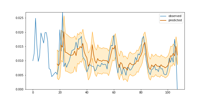
Figure 1. Visit value forecasting with Gaussian process

If the forecast is consistent, approximately 67% of future observations fall within the standard error of the mean. In Figure 1 almost all of observations are within the standard error range, which suggests that the standard error is overestimated. Still, some of the observations which fall outside the standard error range are due to unusual spikes in the observed visit value, either during the preceding hour or on the same hour a day before (the model accounts for daily seasonality). Apparently, some noisy observations negatively affect the quality of forecasting. If we could filter them out or diminish their influence on the overall trend, we would be able to improve forecasting accuracy.

The problem of outliers and varying noise in Gaussian processes is not new, and solutions were proposed in the past. One of the solutions is Student’s t-processes, which are similar to Gaussian processes but are based on the Student’s t-distribution instead of the Gaussian distribution. The Student’s t-distribution has a similar bell-like shape but heavier tails, resulting in unusually deviating measurements having lower influence on the forecast.

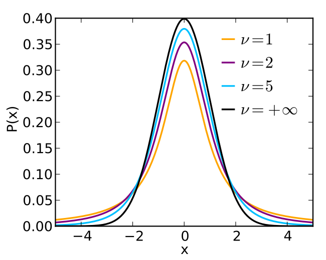
Figure 2. Student-t distribution with different degrees of normality ν (from Wikipedia)

Theoretically, this is a promising solution. There is also an implementation of Student’s t-processes in Python. Practically though, Student’s t-processes are not as flexible in supporting elaborated kernels accounting for different seasonalities, external predictors, or non-stationarity. Gaussian processes are also much more widely adopted and better tested and supported. We would definitely prefer to use Gaussian processes if we could find a way to accommodate for varying noise.

While in general that would be too much to ask for, in the case of visit value forecasting we know the relative noise of different observations, which is proportional to the number of visits over which the average visit value is estimated: the variance of a visit value estimate over an hour with 10 visits will be ten times higher than over an hour with 100 visits. As usually done with Gaussian processes, we estimate the noise factor by maximizing the likelihood of observations, but for each observation we divide the factor by the number of visits. For forecasting, we multiply the observation noise by the average number of visits per observation.

We implemented this ‘weighted noise’ trick for the scikit-learn version of Gaussian processes, using the WhiteKernel as the starting point and modifying the code to accept observation weights. Figure 3 compares forecasting with fixed (orange) and weighted (green) noise. The weighted noise prediction gives much tighter confidence bounds, while still closely following the dynamics of the average visit value.

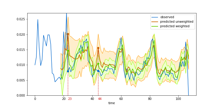
Figure 3. Visit value forecasting with Gaussian process and weighted noise

This addition took only a couple dozen lines of code, including tests, and greatly improved forecasting accuracy. In this case, a simple solution taking into account the structure of data and the process of data collection gave excellent results at a low development and deployment cost.